All Projects

Learning Unions of Convex Sets via
Invertible Latent Decomposition for Path Planning

🎉 Accepted to CoRL 2026

Abstract

Collision-free path planning in cluttered, real-world environments relies on a representation of the collision-free space, and existing representations broadly fall into two categories. Explicit representations, such as unions of convex sets, can be plugged into optimization-based planners as hard collision-free constraints, but their parameters scale poorly with configuration-space dimension. Implicit representations, by contrast, are flexible and scale well to complex geometries, yet typically lack such guarantees. We bridge this gap with ILD (Invertible Latent Decomposition), a framework that jointly learns an invertible mapping and a union of explicit convex polytopes in the resulting latent space. Planning is carried out over these latent convex sets, and the invertible mapping decodes the resulting paths back to the original configuration space while preserving feasibility with respect to the refined explicit safe regions. We further propose Visibility-Guided Sampling (VGS) to keep the convex sets connected for path planning. Across 2D navigation, 6-DoF, and 14-DoF manipulation environments, ILD achieves broader coverage, better inter-set connectivity, and higher path-planning success rates than prior baselines, with zero observed false positives after test-time refinement. On a 14-DoF bimanual manipulator, we further demonstrate real-time collision-free planning, with test-time refinement adapting to scene-geometry changes during real-world deployment on a single 6-DoF arm.


Overview

Explicit representation

e.g. RRT/PRM nodes, Graph of Convex Sets

  • Incorporates hard constraints
  • Locally editable
  • Scales poorly with dimension
ILD bridges both

Implicit representation

e.g. Signed Distance Function

  • Models complex geometry
  • Scales to high dimension
  • No hard feasibility guarantee

Ours: explicit convex sets in a learned, implicit latent space

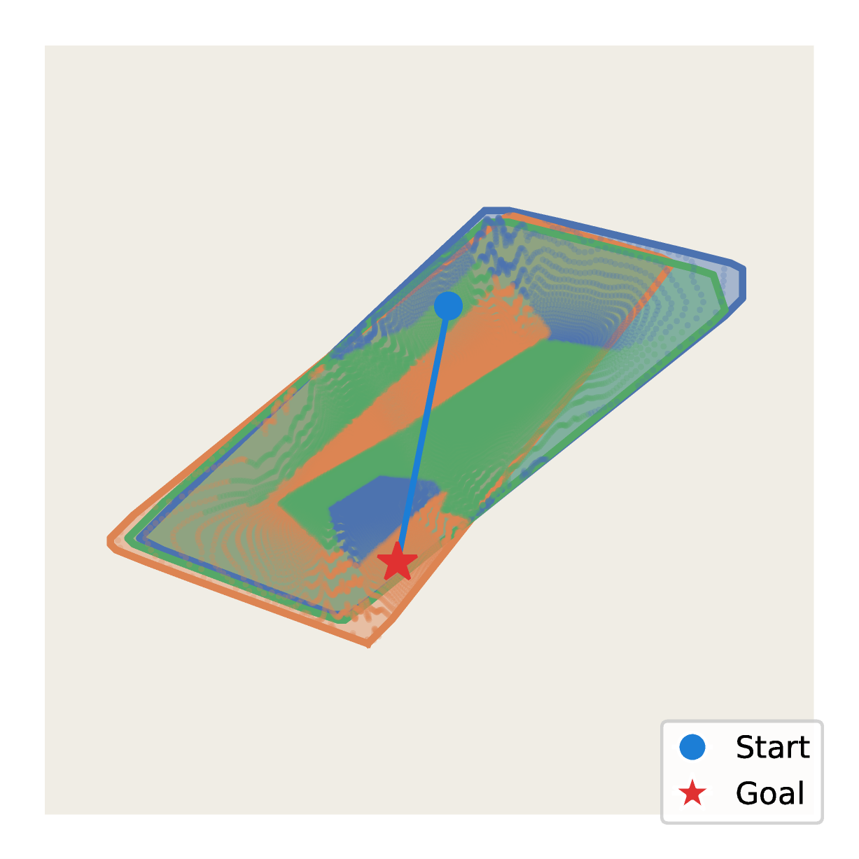
An invertible network deforms the configuration space into a latent space where the collision-free region is a union of convex polytopes. The polytopes stay explicit, the deformation stays implicit, and invertibility keeps the two in one-to-one correspondence.

  • Hard constraints for GCS planning
  • Locally editable at test time
  • Complex geometry with few polytopes
  • Scales to 14-DoF
Environment
Configuration space
Visibility-based seeding
Decomposition in configuration space
$g_\theta$
Invertible
network
$g_\theta^{-1}$
Convex polytopes in latent space
Invertible latent decomposition
Planning in latent space
GCS planning in latent space
Deployment
Decode and deploy

Method

Latent convex decomposition

We model the collision-free space $\hat{\mathcal{Q}}_{\text{free}}$ as the inverse image of a union of convex polytopes $\mathcal{P}_k$ in a learned latent space: $\hat{\mathcal{Q}}_{\text{free}} = g_\theta^{-1}\big(\bigcup_{k=1}^{N} \mathcal{P}_k\big)$, with $\mathcal{P}_k = \{\, \mathbf{z} \mid \boldsymbol{\eta}_{k,i}^{\top}\mathbf{z} + d_{k,i} \ge 0,\ i = 1,\dots,B \,\}$. Here $g_\theta$ is an invertible neural network mapping the configuration space to the latent space, and $\mathcal{H} = \{\boldsymbol{\eta}_{k,i}, d_{k,i}\}$ is a set of hyperplanes. The invertible mapping is the key idea: with an encoder/decoder architecture, a collision-free region in the latent space might not correspond to a collision-free region in the configuration space, whereas an invertible map provides a one-to-one guarantee.

Decomposition cast as a classification problem

phi_0(z)
phi_1(z)
phi_2(z)
$\sigma\big(\max_k \phi_k(\mathbf{z})\big)$
class probability
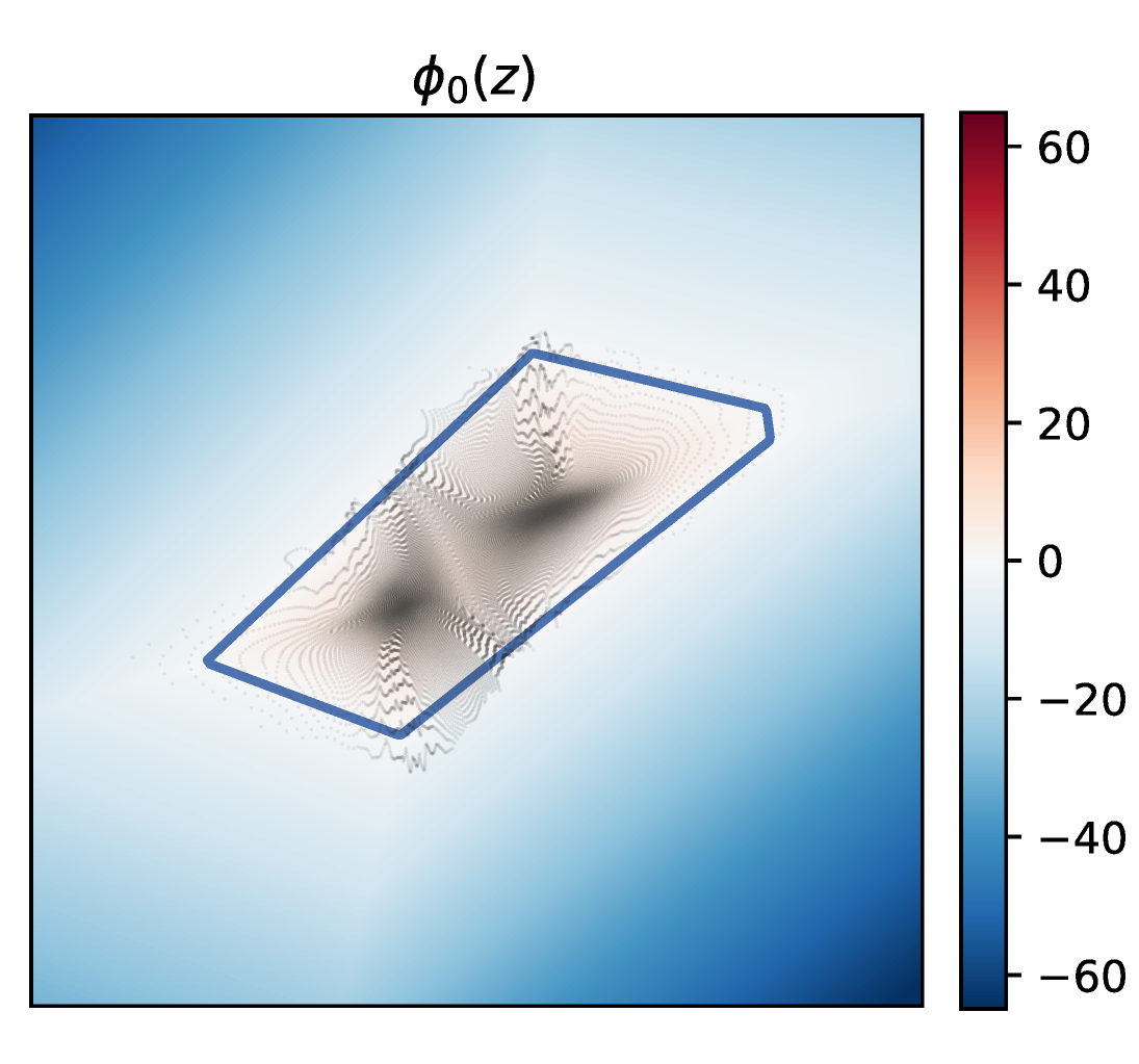
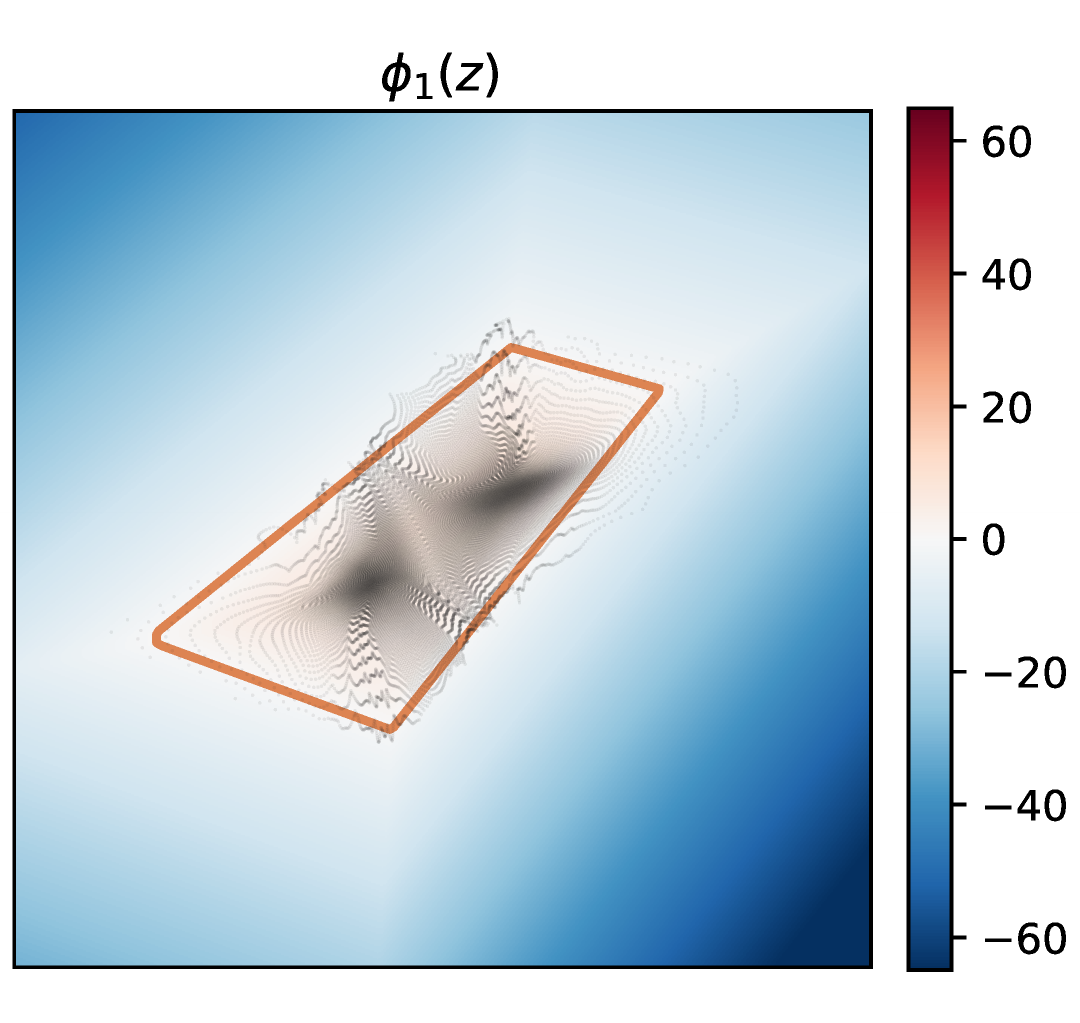
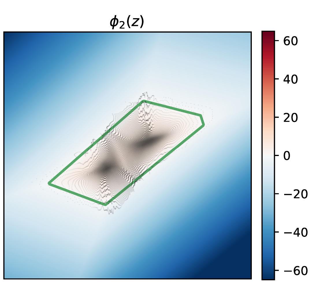
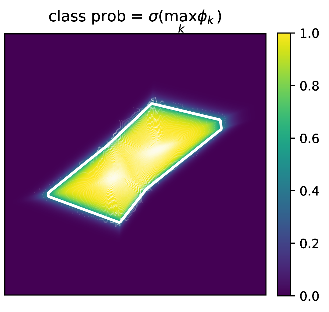
Each polytope $\mathcal{P}_k$ is described by the signed distance $\phi_k(\mathbf{z})$ to its closest boundary. Taking the maximum over polytopes unions them, and a sigmoid turns it into the probability that $\mathbf{z}$ is collision-free. The hyperplanes are thus learned by classifying sampled configurations as safe or unsafe.

Invertible mapping to warp the configuration space

Configuration space
Configuration space $\mathbf{q}$
$g_\theta$
Invertible
network
$g_\theta^{-1}$
Latent space
Latent space $\mathbf{z} = g_\theta(\mathbf{q})$
An invertible neural network $g_\theta$ deforms the configuration space so that the collision-free region becomes a union of convex polytopes. Invertibility guarantees that every latent polytope maps back to a collision-free region in the configuration space.

We jointly optimize $\theta$ and $\mathcal{H}$ with a binary cross-entropy loss on the safe/unsafe labels. To ensure that the shortest path in the latent space matches the shortest path in the configuration space, we add an isometric loss that keeps the two spaces locally distance-preserving.

Visibility-Guided Sampling (VGS)

Seeding

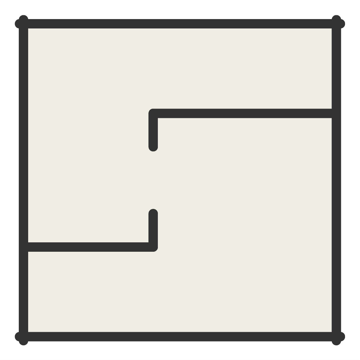
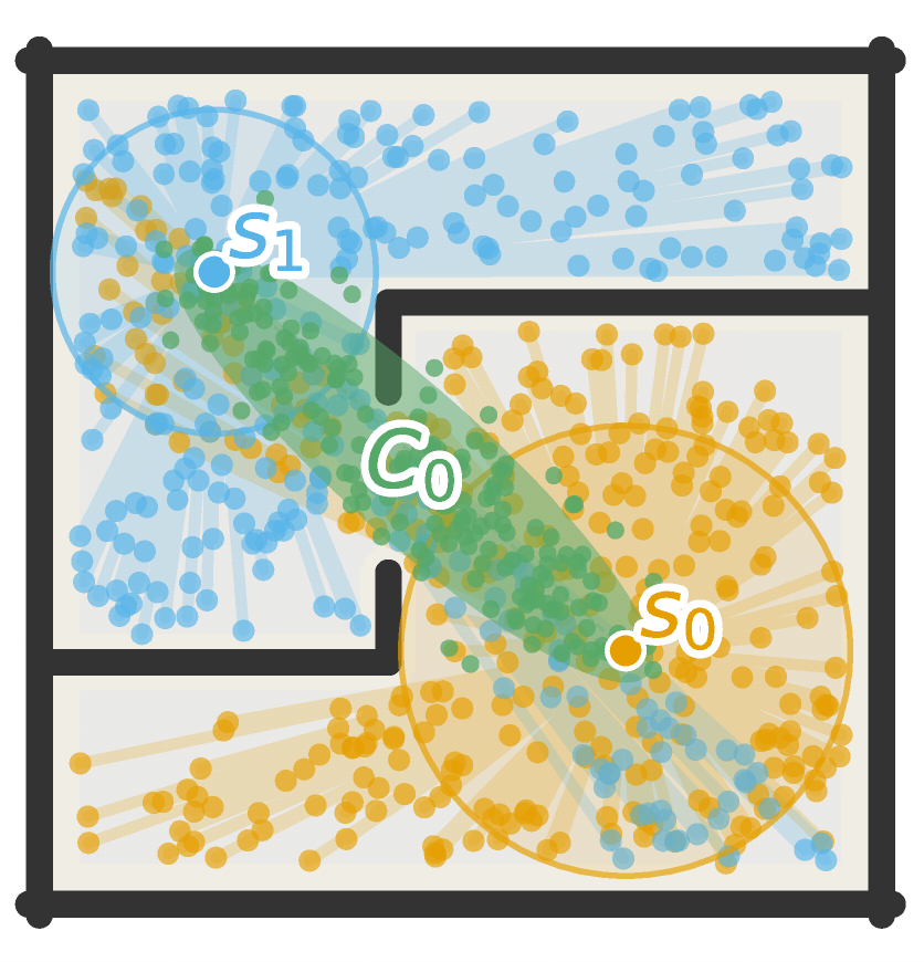
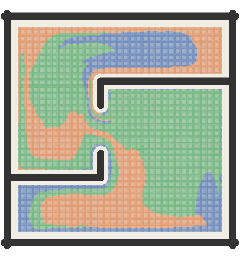
To improve training stability, we encourage each polytope to be responsible for a local region. Since the space is deformed by an invertible network, a set of mutually visible points can be covered by a single polytope in the latent space. We therefore pick seeds $s_0, s_1, \dots$ at points with high visibility, define bridges $C_0$ that connect them, and let each convex polytope cover one of these regions.

Planning in latent space

Given a start and goal, we encode them into the latent space, plan a collision-free path there with a Graph of Convex Sets (GCS) solver, and decode the path back to the configuration space. GCS solves a mixed-integer problem that is relaxed into a convex objective with linear constraints.

Test-time refinement

Test-time refinement
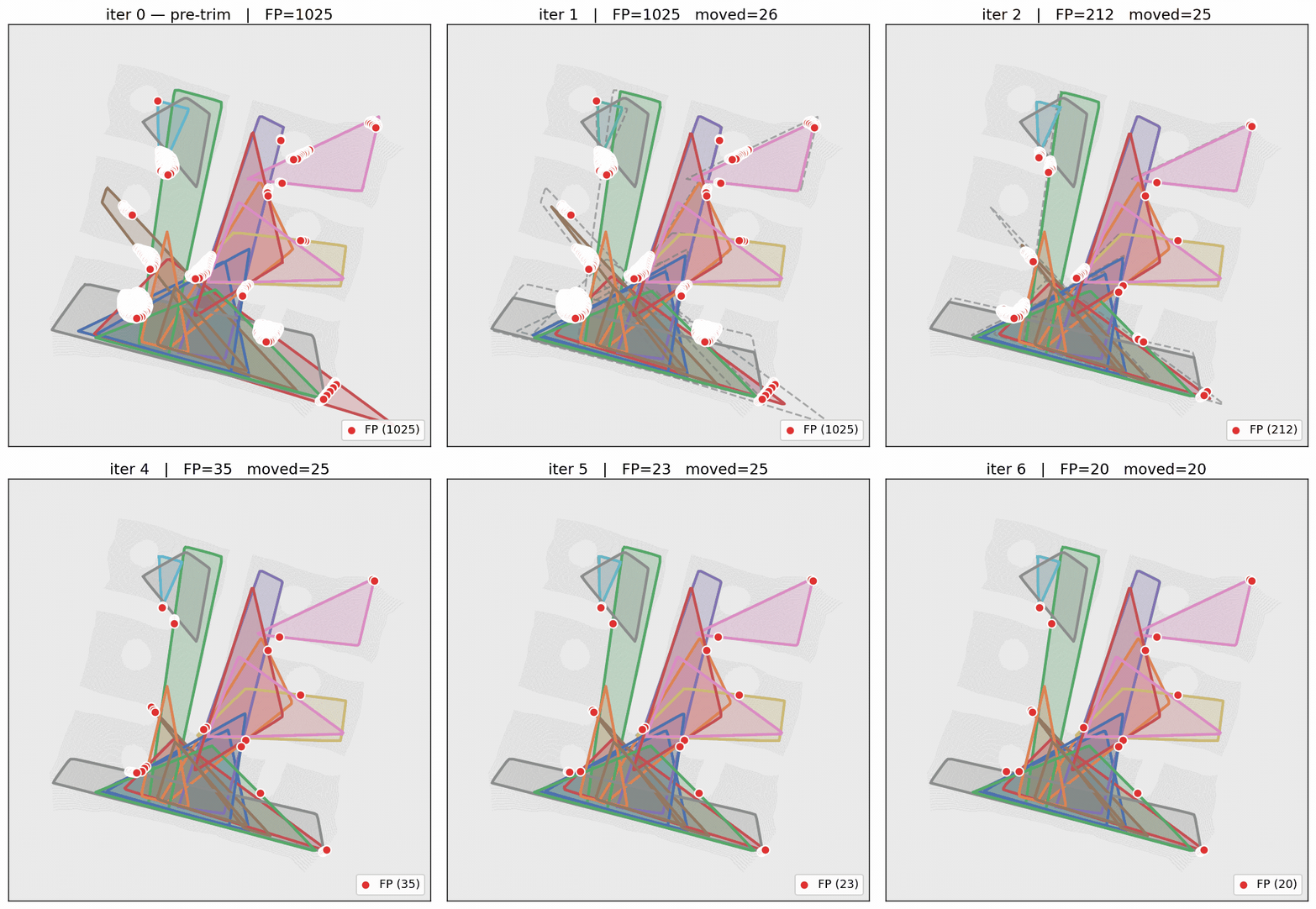
Boundaries are shifted toward the responsible false positives (red), progressively shrinking the unsafe overlap.

A further benefit of an explicit safe-region representation is the ability to correct false positives, regions predicted as safe that are actually unsafe, at test time. For each polytope boundary we move the offset by the worst penetration: $\hat{d}_{k,i} \leftarrow d_{k,i} - \Delta_{k,i}$, where $\Delta_{k,i} = \max_{\mathbf{z}_{\text{fp}} \in \mathcal{F}_{k,i}} \phi_{k,i}(\mathbf{z}_{\text{fp}})$. Repeated application drives the false-positive rate to zero, so collision-induced failures can be eliminated through continual refinement, without retraining.

Results

Fewer convex polytopes, faster planning

3 polytopes
3 polytopes in latent space

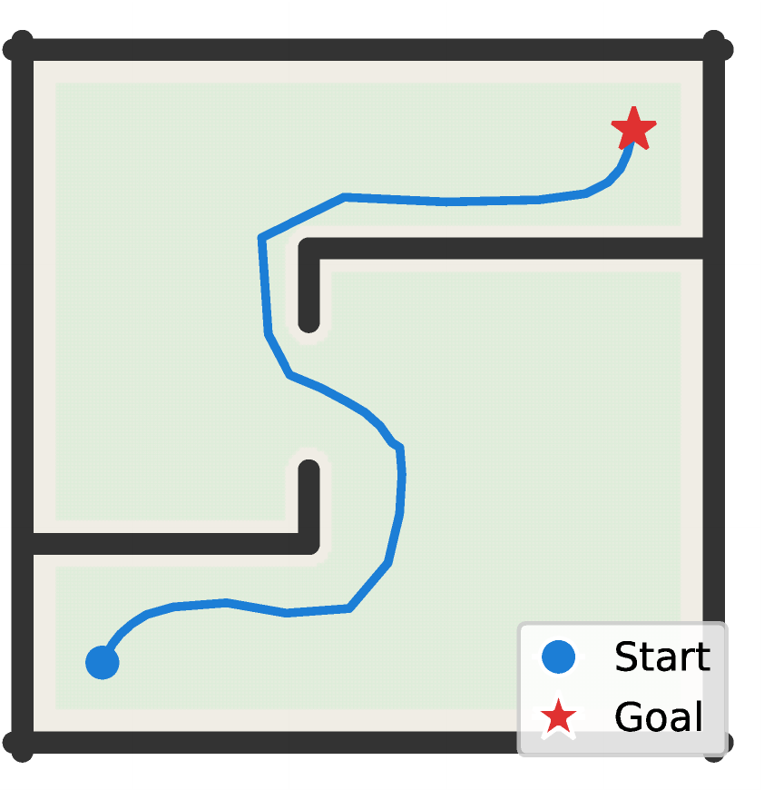
By deforming the space, the collision-free region can be covered with far fewer convex polytopes, enabling faster path planning downstream. In this 2D example, a region that would require nine patches to cover in the configuration space is covered by only three in the latent space. The effect becomes even more pronounced in high dimensions or when the environment is complex. Compared to IRIS, which directly optimizes convex sets in the configuration space and whose solve time grows quickly with dimension, our learning-based decomposition requires fewer convex sets and keeps inference time nearly constant regardless of dimension. Ablations confirm that both the latent model and the visibility-guided sampling contribute substantially to the success rate.

Planning on diverse platforms

2D Navigation

6-DoF Reacher

14-DoF Bimanual

Test-time refinement on a real robot

Test-time refinement also handles modest environment changes without retraining. In the pick-up task the model was trained with a 20 cm wall. We then raise the wall by an additional 10 cm and run a few refinement iterations; the robot successfully avoids the altered obstacle and completes the task.

Original environment

Changed environment (after refinement)

BibTeX